Recently, I think I developed a quite new approach to estimate the distribution of the overlapping backtest pass rates of a brownian motion process over a certain threshold. Say w00t? Read on for explanations…

What typically arises in timeseries models, is that a certain measure is predicted, that should represent the expectancy (or some quantile) of a given timeserie in the future. For example: you’re a very smart person, and you’ve put in place a model that predicts the value of the S&P 500 tomorrow. You want to start trading like a maniac, but your mom tells you to check first if the model actually works over some time, before you put your piggy bank to action.

When I grow up, I will be rich

Now the obvious way to do that, is what is called in financial modelling: “backtesting” the model. For two weeks, you predict the value of the S&P 500 tomorrow, and you check how close it is to that value tomorrow. To keep things simple, you just predict “up” or “down”, and look at whether you were right or not.

This simple exercise illustrates the principle of backtesting for a very simple example, but this is quite close to the way financial institutions and insurers do things.

Now two (business) weeks have passed, and you look at the results: you were right on 8 days! That’s 80%! You quickly start calculating your future wealth, while opening an online trading account and buying a yacht on credit. But mommy comes around and asks you, how sure are you that that wasn’t just luck? You look at the woman’s inability to understand business opportunities in disdain, but the question slowly sinks in and you start fearing the worst. That exhilarating feeling that you were going to be rich slowly crumbles, and you’re stuck thinking about boring stuff again…

Mommy’s right, perhaps this was just plain luck, and the model is actually quite bad, but “happened” to predict correctly by chance during that week… How can I know that? How can I “quantify” that people would say in financial modelling.

Some things, you know for sure: if the model predicts correctly 80% of the time on a very long period of time, it “probably” must be correct, right? Probably correct? How probable? After how long are you confident enough to sacrifice your piggy bank and start trading?

All these questions arise, and have been answered (impecfectly, but still) with the help of statistics. In our earlier example, you could compute the probability that your model is correct in 80% of the times using a backtest and hypothesis testing. You will need to make some assumptions regarding the nature of randomness in the S&P 500, but you will get quite a better answer than trying to figure it out with your “gut feeling”.

Alea jacta est

One of the very important statistical distributions that is used to derive intuitive results from backtests, is the Binomial distribution. Let’s say you have a coin, and it is perfectly symmetric. You have a good understanding of physics, you don’t believe (too much) in God or Fate, so you know that the coin will fall with a probability of 50% with “heads” facing up.

A problem that quickly appears is to know the probability that the coin will fall on heads, exactly K times in N throws. It was understood quite early on that a new toss would be independent from its earlier tosses. I.e. even if the coin was tossed heads ten times, the eleventh time, the probability is still 50% that it falls on heads. This leads to the quite trivial derivation of the Binomial distribution, which mostly resumes to a counting problem (counting all the ways to throw K times heads in N tosses, divided by all the possible outcomes of N tosses).

With the help of this distribution, we can answer in a quite specific way the question we had above: what is the probability to observe the realised backtest given my assumption that my model is correct in 80% of the cases. We observed 8 out of 10 correct predictions. Can we get an idea of how confident we are that the model predicts with an accuracy of 80%? We can compute the probability of observing specific backtest outcomes under this hypothesis with the help of the Binomial distribution. Simple math tools like Excel have the function: BINOM.DIST. The chart below shows the results in a graphical manner.

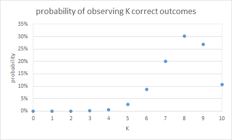
As we can see on that chart, as long as we observe between 5 and 10 correct predictions, we cannot reject the hypothesis that our model is correct 80% of the time, because the probabilities of observing such backtests are not super-low.

A question that would be even better to answer in this case, is what the probability is that the model is right, under the current observations, and this result could be easily derived too, but I want to focus on regular backtesting in this post.

A bit more complex stuff

The result I derived applies to backtesting in a more general setting: estimation of percentiles of a specific random variable. Time-series models typically not only predict averages, but the entire distribution of a specific quantity in the future. In our example above, a classical GBM equity model would predict the value of the S&P 500 in x days as represented in the figure below:

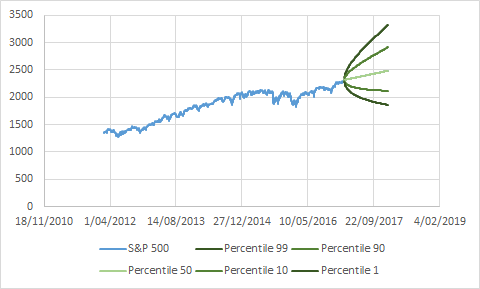
We can see the “envelopes” (percentiles 99, 90, 10 and 1) of the prediction distribution over time in darker and darker green.

Now the way to backtest an entire distribution can be done by testing whether indeed in the realizations of the variable (the S&P in our case), the percentile X is above the realization X percent of the time. So if we observe the S&P 500 over one year, we would expect the percentile 99 estimate to be above the S&P 99% of the time.

Again here, the Binomial distibution can be used to see whether or not the backtest was “likely” under the hypothesis that the prediction model is correct. For example, if we have 100 observations, we should be on average 99 times under percentile 99. With the binomial distribution, we can check again the probability of observing K:

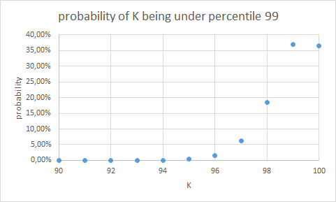
To quantify this in an easy manner, we typically compute the left and right “confidence intervals” (CI) of the number of times we are under percentile X. Typically a 95% CI is used, which is in this case: [97, 100]. I.e. if we observe between 97 and 100 (times below percentile 99), we say the backtest passes, if we observe below or above that (in this case above is impossible, but we can observe e.g. 96 times only below percentile 99, which we will call 4 “excesses”), we say the backtest fails.

A bit even more complex stuff

Now this is all very easy for the case where we just look at one-day predictions. What can happen, however, is that we look at N-day predictions (I will use 10-day to keep things simple here, but results are general). In that case, we cannot apply the Binomial distribution, because: if we predicted today that the percentile 99 of the S&P 500 would be at X in 10 days, and we observe an excess, this will have an obvious impact on what we see tomorrow! Indeed, if we observed an excess this means that the S&P has risen hugely between yesterday and t+9, so it means that our backtest between today and t+10 has much higher probability to be an excess too…

Things become a bit more involved here, so I will formalise things mathematically. Define:

Where:

are the $ lag $-day returns (yes, note that I went a bit fast, but we backtest returns actually, not the serie itself). The small x are just independent random normals:

Now define:

which is the quantity we want to backtest (the sum of excess indicators, i.e. the “backtest results”). This $ S_n $ variable is not distributed Binomially any more, however. Can we still derive confidence intervals for it? The answer is yes, it’s not very easy, but I’ve developed a semi-analytic way of doing it.

The distribution of overlapping-returns backtest excesses

We are going to express the probability mass function (pmf) of $ S_n $ analytically, and then we will see ways to (try) to compute them in practice.

In order to have the pmf of $ S_n $, we first compute the joint distribution of $ Z_i $s . Since we know that $ Z_i $ is independent from $ Z_{i+lag} $, computing the distribution of $ Z_0, Z_1, …, Z_{lag-1} $ is sufficient to describe the joint distribution for any $ i $.

So we define:

where thus: $ \delta_i = +1 $ if $ z_i = 1 $, $ \delta_i = -1 $ otherwise.

We can easily see that:

with

Now, for small $ lag $s, we can evaluate $ P(\delta_0 X_0 \leq \delta_0 K, \delta_1 X_1 \leq \delta_1 K, …, \delta_{lag-1} X_{lag-1} \leq \delta_{lag-1} K) $ analytically. Sadly, it quickly becomes hard, and for $ lag $ as small as 5, crappy Monte-Carlo techniques are needed already…

The result that I derived is the following one: define:

We then can easily compute:

by simply summing the correct probability combinations of $ s_1 = z_0 + z_1 $ in the previous expression. Once we have the above distribution, we can obtain:

by the following property:

and the fact that:

since $ Z_{lag+1} \perp S_1 $ and:

which can be evaluated since we know the numerator (which has the same distribution as $ P(Z_1=z_1, …, Z_{lag}=z_{lag}) $) and the denominator (which can be derived from the same).

We now have evaluated $ (10) $, so we can easily repeat the same grouping step of $ S_1 $ and $ Z_2 $, to obtain :

which can then be used to evaluate:

in the same manner as done above. To summarize these (not very readable, but exhaustive):

Voilà! I actually implemented this procedure in Python in order to have the confidence intervals of any backtest with $ lag $-overlapping returns, and they match Monte-Carlo simulated confidence intervals quite perfectly. Note that to compute the multivariate normal (Gaussian) probabilities, I used scipy’s scipy.stats.mvn.mvnun, which actually also relies on Monte-Carlo sampling techniques when $ lag $ becomes large, so the main advantage of using this method is only that once you have computed the pmfs of a N-day, $ lag $-overlapping backtest once, you can combine and convolute the pmfs of arbitrary N-day, P-day, … backtests and know exactly in what their confidence intervals should be without relying on a heavy Monte-Carlo method each time.